Understanding Cross-Entropy Loss and Focal Loss

Classifications
Output Activation Functions
Losses
- Cross Entropy Loss
- Focal Loss
  - How Focal Loss Works?
    - What is Alpha and Gamma ?
  - Focal Loss: Code Implementation

[Updated on 03-12-2021: Fixed the Focal Loss Code]

In this blogpost we will understand cross-entropy loss and its various different names. Later in the post, we will learn about Focal Loss, a successor of Cross-Entropy(CE) loss that performs better than CE in highly imbalanced dataset setting. We will also implement Focal Loss in PyTorch.

Cross-Entropy loss has its different names due to its different variations used in different settings but its core concept (or understanding) remains same across all the different settings. Cross-Entropy Loss is used in a supervised setting and before diving deep into CE, first let’s revise widely known and important concepts:

Classifications

Multi-Class Classification
One-of-many classification. Each data point can belong to ONE of $C$ classes. The target (ground truth) vector $t$ will be a one-hot vector with a positive class and $C-1$ negative classes. All the $C$ classes are mutually exclusives and no two classes can be positive class. The deep learning model will have $C$ output neurons depicting probability of each of the $C$ class to be positive class and it is gathered in a vector $s$ (scores). This task is treated as a single classification problem of samples in one of $C$ classes.

Multi-Label Classification
Each data point can belong to more than one class from $C$ classes. The deep learning model will have $C$ output neurons. Unlike in multi-class classification, here classes are not mutually exclusive. The target vector $t$ can have more than a positive class, so it will be a vector of $0$ s and $1$ s with $C$ dimensionality where $0$ is negative and $1$ is positive class. One intutive way to understand multi-label classification is to treat multi-label classification as $C$ different binary and independent classification problem where each output neuron decides if a sample belongs to a class or not.

Output Activation Functions

These functions are transformations applied to vectors coming out from the deep learning models before the loss computation. The outputs after transformations represents probabilities of belonging to either one or more classes based on multi-class or multi-label setting.

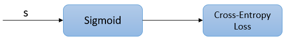
Sigmoid
It squashes a vector in the range $(0,1)$ . It is applied independently to each element of vector $s$ .

f(s_i) = \frac{1}{1 + e^{-s_{i}}}

Softmax
It squashes a vector in the range $(0, 1)$ and all the resulting elements add up to $1$ . It is applied to the output vector $s$ . The Softmax activation cannot be applied independently to each element of vector s, since it depends on all elements of $s$ . For a given class $s_i$ , the Softmax function can be computed as:

f(s)_i = \frac{e^{(s_i)}}{\sum_{j}^C e^{s_j}}

Losses

Cross Entropy Loss

The cross-entropy loss is defined as:

CE = -\sum_i^C t_i log(s_i )

where $t_i$ and $s_i$ are the goundtruth and output score for each class i in C.

Taking a very rudimentary example, consider the target(groundtruth) vector t and output score vector s as below:

Target Vector: [0.6     0.3     0.1]
Score Vector:  [0.2     0.3     0.5]

Then CE will be computed as follows:

CE = -(0.6)log(0.2) - 0.3log(0.3) - 0.1log(0.5) = 0.606

In supervised machine learning settings, elements of target vectors are either 1 or 0. The above example shows how CE is computed and how it is also applicable to find loss between the distributions.

Categorical Cross-Entropy Loss

In multi-class setting, target vector t is one-hot encoded vector with only one positive class (i.e. $t_i = 1$ ) and rest are negative class (i.e. $t_i = 0$ ). Due to this, we can notice that losses for negative classes are always zero. Hence, it does not make much sense to calculate loss for every class. Whenever our target (ground truth) vector is one-hot vector, we can ignore other labels and utilize only on the hot class for computing cross-entropy loss. So, Cross-Entropy loss becomes:

CE = -log(s_i)

The above form of cross-entropy is called as Categorical Cross-Entropy loss. In multi-class classification, this form is often used for simplicity.

The Categorical Cross-Entropy loss is computed as follows:

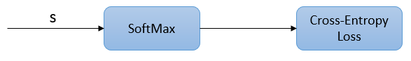
f(s)_i = \frac{e^{s_i}}{\sum_{j}^{C}e^{s_j}} \Rightarrow CE = -\sum_i^C t_i log(f(s)_i) \Rightarrow CE = -log(f(s)_i)

As, SoftMax activation function is used, many deep learning frameworks and papers often called it as SoftMax Loss as well.

Binary Cross-Entropy Loss

Based on another classification setting, another variant of Cross-Entropy loss exists called as Binary Cross-Entropy Loss(BCE) that is employed during binary classification $(C = 2)$ . Binary classification is multi-class classification with only 2 classes. To dumb it down further, if one class is a negative class automatically the other class becomes positive class. In this classification, the output is not a vector s but just a single value. Let’s understand it further.

The target(ground truth) vector for a random sample contains only one element with value of either 1 or 0. Here, 1 and 0 represents two different classes $(C = 2)$ . The output score value ranges from 0 to 1. If this value is closer to 1 then class 1 is being predicted and if it is closer to 0, class 0 is being predicted.

BCE = -\sum_{i=1}^{C=2}t_ilog(f(s)_i) = -t_1log(f(s_1)) - (1-t_1)log(1-f(s_1))

$s_1$ and $t_1$ are the score and groundtruth label for the class $C_i$ in $C$ . $s_2 = 1 -s_1$ and $t_2 = 1 - t_1$ are the score and groundtruth label for the class $C_2$ . If $t_1 = 0$ then $-t_1log(f(s_1))$ would become $0$ and $(1-t_1)log(1-f(s_1))$ would become active. Similarly, if $t_1 = 1$ then $-t_1log(f(s_1))$ would become active and $(1-t_1)log(1-f(s_1))$ would become $0$ . The loss can be expressed as:

CE = \begin{cases} -log(f(s_1)) & if & t_1 = 1 \\ -log(1-f(s_1)) & if & t_1 = 0 \end{cases}

To get the output score value between [0,1], sigmoid activation function is used.

Due to the using of Sigmoid Activation function it is also called as Sigmoid-Cross Entropy Loss.

f(s_1) =\frac{1}{1+e^{-s_1}} \Rightarrow CE = -t_1log(f(s_1)) - (1-t_1)log(1-f(s_1))

Cross-Entropy in Multi-Label Classification

As described earlier, in multi-label classification each sample can belong to more than one class. With $C$ different classes, multi-label classification is treated as $C$ different independent binary classification. Multi-label classification is a binary classification problem w.r.t. every class. The output is vector $s$ consisting of $C$ number of elements. Binary Cross-Entropy Loss is employed in Multi-Label classification and it is computed for each class in each sample.

Loss = \sum_{i=1}^{i=C}BCE(t_i, f(s)_i) = \sum_{i=1}^{i=C}t_ilog(f(s)_i)

Focal Loss

Focal Loss was introduced in Focal Loss for Dense Object Detection paper by He et al (at FAIR). Object detection is one of the most widely studied topics in Computer Vision with a major challenge of detecting small size objects inside images. Object detection algorithms evaluate about $10^4$ to $10^5$ candidate locations per image but only a few locations contains objects and rest are just background objects. This leads to class imbalance problem.

Using Binary Cross-Entropy Loss for training with highly class imbalance setting doesn’t perform well. BCE needs the model to be confident about what it is predicting that makes the model learn negative class more easily they are heavily available in the dataset. In short, model learns nothing useful. This can be fixed by Focal Loss, as it makes easier for the model to predict things without being $80-100%$ sure that this object is something. Focal Loss allows the model to take risk while making predictions which is highly important when dealing with highly imbalanced datasets.

Though Focal Loss was introduced with object detection example in paper, Focal Loss is meant to be used when dealing with highly imbalanced datasets.

How Focal Loss Works?

Focal Loss is am improved version of Cross-Entropy Loss that tries to handle the class imbalance problem by down-weighting easy negative class and focussing training on hard positive classes. In paper, Focal Loss is mathematically defined as:

$Focal Loss = -\alpha_t(1 - p_t)^{\gamma}log(p_t)$

The above definition is Focal Loss for only one class. It has omitted the $$\sum$$ that would sum over all the classes $$C$$. To calculate total Focal Loss per sample, sum over all the classes.

What is Alpha and Gamma ?

The only difference between original Cross-Entropy Loss and Focal Loss are these hyperparameters: alpha( $\alpha$ ) and gamma( $\gamma$ ). Important point to note is when $\gamma = 0$ , Focal Loss becomes Cross-Entropy Loss.

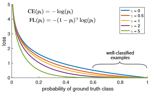
Let’s understand the graph below which shows what influences hyperparameters $\alpha$ and $\gamma$ has on Focal Loss and in turn understand them. In the graph, “blue” line represents Cross-Entropy Loss. The X-axis or “probability of ground truth class” (let’s call it pt) is the probability that the model predicts for the ground truth object. As an example, let’s say the model predicts that something is a bike with probability $0.6$ and it actually is a bike. In this case, pt is $0.6$ . In the case when object is not a bike, the pt is $0.4 (1-0.6)$ . The Y-axis denotes the loss values at a given pt.

As can be seen from the image, when the model predicts the ground truth with a probability of $0.6$ , the Cross-Entropy Loss is somewhere around $0.5$ . Therefore, to reduce the loss, the model would have to predict the ground truth class with a much higher probability. In other words, Cross-Entropy Loss asks the model to be very confident about the ground truth prediction.

This in turn can actually impact the performance negatively:

The deep learning model can actually become overconfident and therefore, the model wouldn’t generalize well.

Focal Loss helps here. As can be seen from the graph, Focal Loss with $\gamma > 1$ reduces the loss for “well-classified examples” or examples when the model predicts the right thing with probability $> 0.5$ whereas, it increases loss for “hard-to-classify examples” when the model predicts with probability $<0.5$ . Therefore, it turns the model’s attention towards the rare class in case of class imbalance.

$\gamma$ controls the shape of curve. The higher the value of $\gamma$ , the lower the loss for well-classified examples, so we could turn the attention of the model towards ‘hard-to-classify’ examples. Having higher $\gamma$ extends the range in which an example receives low loss.

Another way, apart from Focal Loss, to deal with class imbalance is to introduce weights. Give high weights to the rare class and small weights to the common classes. These weights are referred as $\alpha$ .

But Focal Loss paper notably states that adding different weights to different classes to balance the class imbalance is not enough. We also need to reduce the loss of easily-classified examples to avoid them dominating the training. To deal with this, multiplicative factor $(1-p_t)^{\gamma}$ is added to Cross-Entropy Loss which gives the Focal Loss.

Focal Loss: Code Implementation

Here is the implementation of Focal Loss in PyTorch:

class WeightedFocalLoss(nn.Module):
    def __init__(self, batch_size, alpha=0.25, gamma=2):
        super(WeightedFocalLoss, self).__init__()

        if alpha is not None:
            alpha = torch.tensor([alpha, 1-alpha]).cuda()
        else:
            print('Alpha is not given. Exiting..')
            exit()
        
        # repeating the 'alpha' object declared above 'batch_size' times.
        self.alpha = alpha.repeat(batch_size, 1)
        self.gamma = gamma

    def forward(self, inputs, targets):
        # computed BCE loss. This loss function take logits as the inputs i.e. no sigmoid is applied
        BCE_loss = F.binary_cross_entropy_with_logits(inputs, targets, reduction='none')

        # converting type of targets to torch.long
        targets  = targets.type(torch.long)

        # 'gather' api takes input 1 as dimension and targets.data as the index (which are 1 and 0 as targets contains 1 and 0 only).
        # 'gather' creates tensor of size 'targets' (i.e. batch_size x ros_size).
        # each element's value is self.alpha[targets.data] i.e. based on 1 or 0 in targets, alpha's corresponfing index value is taken.
        at       = self.alpha.gather(1, targets.data)

        # Creating the probabilities for each class from the BCE loss.
        pt       = torch.exp(-BCE_loss)

        # Focal Loss formula
        F_loss   = at*(1-pt)**self.gamma * BCE_loss

        return F_loss.mean()

References